I Tried Newton-Muon. The Training Loss Lied to Me.
A small reproduction of Newton-Muon on Tiny Shakespeare, and why training loss can be a dangerously misleading signal when comparing optimizers.
There is a point during an experiment where the result looks obvious. For me, that point was somewhere around the first 1,000 training steps. I was comparing three optimizers on the same small transformer: AdamW, Muon, and Newton-Muon. The model, the dataset, and the random seed were all the same. Only the update rule changed, and Muon looked like it was winning.
At step 1,000, its training loss had already dropped to 1.25. AdamW was at 1.61. Newton-Muon was at 1.54. By the end of training, the difference looked even more ridiculous.
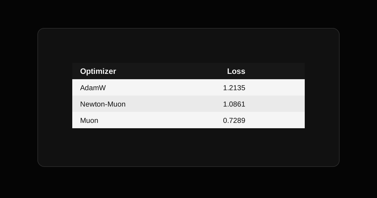
| Optimizer | Final Training Loss |
|---|---|
| AdamW | 1.2135 |
| Newton-Muon | 1.0861 |
| Muon | 0.7289 |
If I had stopped there, this would have been a very different post. Muon had driven the training loss much lower than either AdamW or Newton-Muon. But the model was also being evaluated on data it had not trained on. And there, the story completely changed. Muon wasn't winning. It was overfitting.
How I Ended Up Testing Newton-Muon
I came across Newton-Muon during an ML Collective G-Africa reading session. One of the things I liked about the reading sessions was that we did more than just read and discuss a paper. For each paper, someone took on the role of the "hacker." The hacker's job was to take the experiment described in the paper and try to replicate it, usually at a much smaller scale and with the compute available to us. That week, I was the hacker. So while we were reading and discussing Newton-Muon, my job was to actually make a smaller version of the experiment run.
That distinction is important. I wasn't trying to reproduce every number in the paper. I wasn't training a large language model at the scale used by the authors, and this wasn't meant to establish a new optimizer benchmark. The question was much smaller:
Can I implement the central idea behind Newton-Muon, put it beside Muon and AdamW on the same small language model, and observe what actually changes?
That eventually became a 3.23 million parameter character-level transformer trained on Tiny Shakespeare. Small enough to run on a single Tesla T4. Large enough, I hoped, for differences between the optimizers to become visible. Before getting to the experiment, though, I had to understand what exactly I was implementing. And that starts with Muon.
First, What Is Muon Actually Doing?
Most introductions to optimization start with some variation of gradient descent. You have parameters , calculate their gradient , and update the parameters in the opposite direction:
where is the learning rate. The intuition is straightforward: the gradient tells us which direction increases the loss, so we move in the opposite direction. Of course, the optimizers we actually use are more sophisticated. Adam, for example, keeps moving averages of the gradient and squared gradient, and AdamW separates weight decay from the gradient update. But there is another interesting detail here: a lot of the important parameters inside neural networks aren't just arbitrary collections of independent numbers. They are matrices.
A linear layer, for example, might have a weight matrix:
Its gradient has the same matrix structure:
Muon takes that matrix structure seriously. Rather than treating the update only as a collection of individual scalar parameter updates, Muon performs an operation on the gradient matrix itself. At the center of this is the matrix sign operation.
Suppose we decompose a matrix using singular value decomposition:
The matrix sign is:
The singular values. The operation keeps the singular directions represented by and , while effectively replacing the singular values.
That gives Muon a matrix-aware update instead of applying an independent adaptive rule to every element of the weight matrix. There is a practical problem, though: we don't want to perform a full singular value decomposition every time the optimizer updates a weight matrix.
So Muon approximates this operation using Newton-Schulz iterations.
My implementation used five iterations:
def newton_schulz(G, steps=5):
    a, b, c = (3.4445, -4.7750, 2.0315)

    X = G.bfloat16() / (G.norm() + 1e-7)

    if G.size(0) > G.size(1):
        X = X.T

    for _ in range(steps):
        A = X @ X.T
        X = a * X + b * A @ X + c * A @ A @ X

    if G.size(0) > G.size(1):
        X = X.T

    return X.to(G.dtype)
The gradient is normalized first, converted to bfloat16, and then repeatedly transformed using matrix multiplications. The result becomes the update applied to the weight matrix.
My Muon implementation also maintained momentum:
if s['buf'] is None:
    s['buf'] = G.clone()
else:
    s['buf'].mul_(self.momentum).add_(G)

update = newton_schulz(s['buf'])
So far, so good. But Newton-Muon asks an interesting question. What if the gradient isn't enough?
The Information Muon Doesn't Use
Consider a linear layer. It receives some input , applies its weight matrix, and produces an output. The gradient tells us how changing the weights affects the loss. But the inputs passing through that layer have structure too.
Some directions in the input space may occur frequently. Others may be rare. Some may be highly correlated. Two gradients could therefore look similar while coming from very different input distributions. Newton-Muon tries to account for this.
For a layer receiving activations , we can calculate an input second-moment matrix:
where is the number of activation samples represented in . Instead of immediately giving the raw gradient to Muon, Newton-Muon first right-preconditions it:
Then the usual Muon-style operation happens. The simplified version of the update I implemented was basically three lines:
G_pre  = G @ K_inv
buf    = momentum * buf + G_pre
update = newton_schulz(buf)
That first line is the important difference. Muon sees the gradient. Newton-Muon first changes that gradient using information about the inputs flowing through the layer. At least conceptually, that sounds simple. Implementing it meant I suddenly needed something a normal optimizer doesn't usually need access to: activations.
Getting the Activations Into the Optimizer
The optimizer normally sees parameters and gradients. Newton-Muon also needed .
So I registered forward hooks on the linear layers of the transformer. Each time data passed through one of those layers, the hook captured the input activations:
class ActivationStore:
    def __init__(self):
        self.value = None

    def hook_fn(self, module, input, output):
        x = input[0].detach().float()
        self.value = x.reshape(-1, x.shape[-1]).T
Now the optimizer could access the latest input activations for each linear layer. From those activations, I computed:
I didn't simply replace the previous estimate each time. Instead, I maintained an exponential moving average:
with:
Then came another practical problem: Newton-Muon needs .
Directly inverting a matrix that might be poorly conditioned isn't something I wanted to do without some stabilization. So I added damping based on the average diagonal scale of :
gval = self.gamma * K.trace().item() / n
K_damp = K + gval * torch.eye(n, device=K.device)
with:
and then:
K_inv_new = torch.linalg.inv(K_damp)
I also didn't recompute these inverses at every training step. I refreshed them every 32 steps.
That was an important practical compromise because these matrices could be fairly large. Some of the ones printed during training were .
So my Newton-Muon implementation wasn't just "Muon plus one matrix multiplication." There was now activation capture, second-moment estimation, damping, matrix inversion, caching, and periodic refreshing. Which made the next question obvious: was any of this going to make a visible difference?
Building a Small Test
For the dataset, I used Tiny Shakespeare. It contains 1,115,394 characters of Shakespeare plays concatenated into one text file. I deliberately kept the tokenization simple. Every unique character became a token. No BPE. No subword tokenizer. No pretrained tokenizer. There were only 65 possible tokens.
The data was split 90/10:
Training tokens:   1,003,854
Validation tokens:   111,540
Vocabulary size:           65
Each training example contained a sequence of 128 characters, and the model learned to predict the next character. The model itself was a small GPT-style transformer:
Parameters:       3,225,600
Embedding size:         256
Attention heads:          4
Transformer layers:       4
Context length:         128
Batch size:              64
The transformer block contained multi-head causal self-attention followed by an MLP with GELU activations, with LayerNorm and residual connections around them. Nothing enormous.
The whole thing fit comfortably on the Tesla T4 available in the Kaggle environment:
Tesla T4
VRAM: 15.6 GB
And importantly, the architecture stayed the same for all three experiments. I wasn't comparing different models. I was comparing what happened when the same model was trained using different update rules.
AdamW vs Muon vs Newton-Muon
I used three optimizer configurations. The first was AdamW. This was the familiar baseline, with:
learning rate = 3e-4
weight decay  = 0.1
For Muon and Newton-Muon, there was an important implementation detail. Not every parameter in the transformer went through the matrix optimizer. The linear weight matrices were handled by Muon or Newton-Muon, while parameters such as embeddings, biases and the output head continued to use AdamW.
For Muon, I used:
learning rate = 0.01
momentum      = 0.95
weight decay  = 0.01
For the Newton-Muon run in the builder, I used:
learning rate      = 0.004
momentum           = 0.95
weight decay       = 0.01
beta               = 0.95
gamma              = 0.15
inverse refresh    = every 32 steps
Newton-Schulz      = 5 iterations
One thing worth pointing out is that these are not identical hyperparameters across all three optimizers. So this isn't a controlled claim that one algorithm is universally better than another under every possible tuning. This was a small replication experiment with specific configurations. That distinction matters when we get to the results.
Running the Experiment
Each model started from the same random seed:
torch.manual_seed(42)
Each optimizer trained for 4,000 steps. The training loop itself was deliberately ordinary:
get batch
    ↓
forward pass
    ↓
cross-entropy loss
    ↓
backpropagation
    ↓
gradient clipping
    ↓
optimizer step
I clipped the gradient norm to 1.0. Every 200 steps, I paused to estimate validation loss over 50 held-out batches. That gave me two measurements throughout training. Training loss told me how well the model was fitting the data it was learning from. Validation loss told me how well that learning was transferring to held-out data. And this distinction ended up becoming the most interesting part of the entire experiment.
At First, Muon Looked Great
Muon moved quickly. At step 200:
AdamW        train 2.3429
Muon         train 1.8435
Newton-Muon  train 2.4270
Muon was already substantially ahead on training loss. At step 400:
AdamW        train 2.0170
Muon         train 1.5037
Newton-Muon  train 2.1671
At step 1,000:
AdamW        train 1.6095
Muon         train 1.2501
Newton-Muon  train 1.5431
If I were watching only that number, there wouldn't have been much of a story. Muon was fitting the training set aggressively, and it kept doing so.
By step 2,000:
AdamW        1.3652
Muon         1.0066
Newton-Muon  1.2670
At step 3,000:
AdamW        1.2919
Muon         0.8722
Newton-Muon  1.1913
And finally, at step 4,000:
AdamW        1.2135
Muon         0.7289
Newton-Muon  1.0861
Muon's training loss was nowhere near the others. It looked dominant. Then I plotted validation loss.
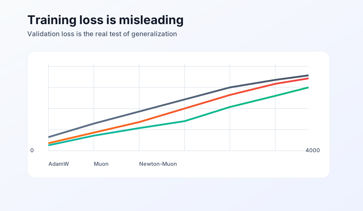
Validation Loss Told a Completely Different Story
At step 1,000, Muon's validation loss reached:
That turned out to be its best validation result in the entire run. Training continued. The training loss kept dropping, but validation loss stopped following it.
At step 1,200:
Then:
Then:
Then:
Then:
And by step 4,000:
Meanwhile, Muon's training loss had fallen all the way to:
This was the interesting part. The optimizer was getting increasingly good at reducing the objective on the training data while its performance on held-out data was getting worse. The gap kept widening. Newton-Muon behaved differently.
Its validation loss started worse than Muon's:
Step 200
Muon         1.9895
Newton-Muon  2.4815
But Newton-Muon kept improving after Muon had already reached its best validation point. At step 1,400:
At step 1,800:
At step 2,000:
At step 2,200:
And at step 2,400:
That was the lowest validation loss reached by any of the three models during this experiment. After step 2,400, Newton-Muon also started moving in the wrong direction. At step 2,600, validation loss rose to 1.5600. At step 3,200 it was 1.5741. By step 4,000 it had reached 1.6211. So Newton-Muon did not eliminate overfitting.
It delayed the point at which the best validation result occurred in this run, and its best checkpoint generalized slightly better than the best checkpoints from the other two configurations.
That wording is important. From this experiment alone, I can't say that Newton-Muon's preconditioner universally acts as a regularizer, or that Newton-Muon will always generalize better than Muon. What I can say is what I observed. Under this setup, Muon's best validation checkpoint appeared at step 1,000. Newton-Muon's appeared at step 2,400. And Newton-Muon's best validation loss was lower.
Putting the Numbers Together
Here is the full summary:
| Optimizer | Final Train Loss | Best Val Loss | Best Val Step | Final Val Loss | Runtime |
|---|---|---|---|---|---|
| AdamW | 1.2135 | 1.5404 | 3,800 | 1.5431 | 363.9s |
| Muon | 0.7289 | 1.5639 | 1,000 | 2.0813 | 465.4s |
| Newton-Muon | 1.0861 | 1.5349 | 2,400 | 1.6211 | 444.6s |
There are several different stories hiding in this table. If the metric is final training loss, Muon wins by a lot. If the metric is the lowest validation loss observed during the run, Newton-Muon has the lowest number, although the difference from AdamW is small:
That is only about a 0.36% reduction relative to AdamW's best validation loss. So I wouldn't look at these numbers and declare that Newton-Muon destroyed AdamW. It didn't. The more interesting difference was the shape of training. Muon reached its best validation loss very early and then continued driving down training loss while validation performance deteriorated.
Newton-Muon followed a different trajectory. Its best validation point arrived 1,400 steps later than Muon's.
AdamW was the slowest of the three in terms of reducing training loss, but its validation behavior was much more stable. Its best validation result came near the end of training, at step 3,800, and its final validation loss of 1.5431 was still close to that minimum.
In fact, if we compare the models at exactly the final step rather than choosing their best checkpoints, AdamW had the lowest validation loss:
AdamW        1.5431
Newton-Muon  1.6211
Muon         2.0813
That is why "which optimizer won?" is actually the wrong question for this experiment. The answer depends on what you measure and when you measure it.
Faster Optimization Didn't Mean Faster Wall-Clock Training
There was another thing I wanted to look at: time. Muon and Newton-Muon perform matrix operations that AdamW doesn't. Newton-Muon goes even further by maintaining activation statistics and periodically computing matrix inverses. So I tracked wall-clock time alongside validation loss.
For 4,000 steps:
AdamW         363.9 seconds
Newton-Muon   444.6 seconds
Muon          465.4 seconds
AdamW was the fastest in this implementation. Newton-Muon finished about 80.7 seconds later than AdamW. Muon took about 101.5 seconds longer than AdamW.
Interestingly, Newton-Muon was slightly faster than my Muon run overall, despite doing the additional preconditioning work. But I would be careful about reading too much into that from a single Kaggle run.
GPU scheduling, implementation details, kernel behavior and other runtime noise can affect timings. The main thing this tells me is that, in this small implementation, neither matrix optimizer gave me a wall-clock advantage over AdamW simply by existing. Again, this is why small replications are useful. An optimizer can be mathematically interesting and still have practical costs that only become obvious when you implement it.
Then I Asked Them to Write Shakespeare
Numbers are the actual measurement here. But because this was a language model, I wanted to look at the models themselves too. So after training, I gave each one the same starting text:
ROMEO:
and sampled another 200 characters.
AdamW produced:
ROMEO:
Far a white tidings of laments!

Second Citizen:
He that once my lappiness I do stood.

PAULINA:
Go, dangerous
What laugh not with hours that saw the rest; here command,
Shall is he in with wun reven
Muon produced:
ROMEO:
Be not so to move our children, thou?

MERCUTIO:
Nay, like your limitations are to be sauced
one: ay, by the voices, whose censure
Dignitions messerity, to bring him to you,
and we should not go not
Newton-Muon produced:
ROMEO:
Nay, no; I say, no, no.
Thou as Titus, Aufidius, and soldiers,
So much as Bolingbroke: that would yourself
I do know; doubt how much adverses! haplot thee
Still we forswords at age, for womb your gue
There are some fun differences. The Newton-Muon sample mentions Titus, Aufidius and Bolingbroke. The Muon model gives us words like "Dignitions" and "messerity." AdamW gives us "lappiness" and "wun." But I don't want to pretend these three samples prove anything that the validation measurements didn't. Generation is stochastic. A different random sample could make one model look better or worse. So I see this part as a qualitative check, not the result of the experiment. The validation curves are much more useful.
The Part I Nearly Got Wrong
This experiment also reminded me of something embarrassingly easy to forget when training models: a falling training loss is not the same thing as improving generalization. That sounds obvious when written down. It becomes less obvious when you're watching an optimizer produce a beautiful curve.
Muon's training loss went:
If that is the only curve on your screen, everything looks great. But after step 1,000, its validation curve was already telling another story. The optimizer continued becoming better at the objective it was being shown while becoming worse on the held-out split. That doesn't mean the training loss "lied" in the literal sense. It answered exactly the question it was supposed to answer. The problem was asking it to answer a question it couldn't. Training loss tells me how well the model is fitting its training data. It does not, by itself, tell me how well that model will generalize. And that distinction became the central result of my replication.
So, Did I Replicate Newton-Muon?
At the scale I was working at, I implemented the central mechanism I set out to test:
I captured layer activations, maintained their second-moment estimates, damped and inverted those matrices, and used them to right-precondition the gradients. Then I passed those gradients through the same Newton-Schulz-based matrix-sign approximation used in my Muon implementation and compared the result against Muon and AdamW on the same small language-model task. What happened was not simply "Newton-Muon won." Muon optimized the training objective much more aggressively. AdamW was cheaper in wall-clock time in my implementation and remained remarkably stable on validation data. Newton-Muon produced the lowest best validation loss of the three runs, at 1.5349, and reached that point later in training than Muon reached its own best validation checkpoint. Those are the results. Anything beyond that needs more experiments.
What I Would Test Next
If I were extending this beyond the reading-session replication, the first thing I would want is multiple seeds.
This experiment used:
torch.manual_seed(42)
One seed is enough to see interesting behavior, but it isn't enough to tell me how consistent that behavior is.
The 0.0055 difference between Newton-Muon's and AdamW's best validation losses is particularly small. I would want to know whether it persists across several independent runs or disappears into run-to-run variation.
I would also tune the optimizers independently rather than treating the configurations in this notebook as their final forms. The learning rates were different. Their weight-decay settings were different. Newton-Muon introduced its own parameters such as , , and the inverse-refresh interval. Those choices matter.
I would want to vary the Newton-Muon refresh interval too. I used 32 steps because constantly recomputing inverses would be expensive.
But that creates another question:
How stale can the estimate of become before the preconditioner stops being useful?
Then there is scale. Tiny Shakespeare and a 3.23M parameter transformer made this experiment possible on a single T4, which was exactly what I needed for a small replication. But it is still Tiny Shakespeare and a 3.23M parameter transformer. Behavior at this scale doesn't automatically transfer to models hundreds or thousands of times larger. That is not a weakness of doing the experiment. It is just the boundary of what the experiment tells me.
What I Took Away From It
I started this because it was my turn to be the hacker. There was a paper being discussed in an ML Collective G-Africa reading session, and my role that week was to take the idea out of the paper and see if I could make a smaller version of the experiment work. That forced me to understand Newton-Muon differently. Reading:
is one thing. Actually implementing it means asking where comes from, how to capture those activations without keeping an unnecessary computation graph alive, how large becomes, why you probably do not want to invert that matrix every step, when to damp it before inversion, what to do when the inverse looks numerically unreasonable, and which parameters should even be handled by the matrix optimizer instead of staying with AdamW. And then, after all of that, it means watching Muon race ahead on training loss and realizing that the most impressive-looking number in the notebook isn't necessarily the one you should care about. That is probably my favorite thing about replication. A paper gives you the idea. Trying to reproduce it forces you to deal with everything between the equation and the result. And sometimes, that space is where the interesting part actually is.


